Turning your Raspberry Pi into a Cloud-Connected Thermostat

2019-01-09

technology

• 11 Minute Read

Temperature Dashboard

Vision

This fall I moved into a new house, which I quickly learned has an extremely unreliable thermostat. As someone who likes to be cool in the evening for bedtime, but also doesn’t love wearing sweaters indoors, I wondered if there might be a better way of monitoring my house’s temperature.

Fortunately for me, I had a surplus Raspberry Pi lying around, which I quickly determined could be leveraged into serving as the brains of my thermostat, given the right input sensors. Plus, the Pi easily connects to the AWS IoT interface, which would allow me to transmit data to AWS and then process and save that data in a variety of locations for analysis.

Here’s the final architecture for the solution I ended up building:

Raspberry Pi reads in temperature data every ten seconds and transmit to an AWS IoT message topic
AWS IoT sends messages from the Pi to a Kinesis Firehose stream
The Firehose should write data in batches to CSV files in an S3 bucket
Athena should crawl the schema of the temperature data in S3 and make the data queryable
Some small SQL queries which run on Athena and aggregate sensor data by hour and day
Hourly, Daily, and Weekly temperature plots for my house in dashboard form, built in Shiny and available on the internet

If you’re interested in building something similar, feel free to steal from the setup details below!

Hardware Requirements

Raspberry Pi with GPIO pins
Breadboard and cables
DS18B20 Temperature Sensor
4.7K or 10k Ohm resistor

Install Temperature Sensor

I’m not a sensor and smart devices guru, so it took some trial-and-error to get my sensor properly connected with my breadboard and Pi. I recommend referring to other setup guides online and testing what might work best for you, but it is totally expected that this step might be a bit tricky!

My Configuration

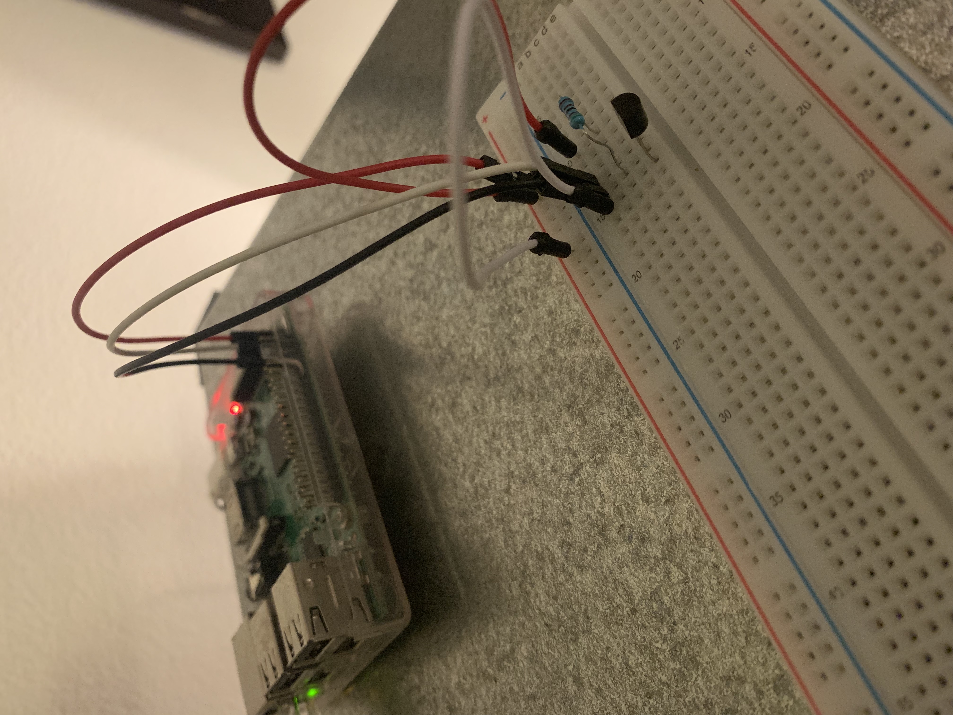
Raspberry Pi with Breadboard and Sensor

Helpful Graphic from Adafruit - Your Mileage May Vary

Helpful graphic from Adafruit

Read Temperature

Once the sensor is installed, you can use the Raspberry Pi’s GPIO interface to read in the sensor data. The script below is a simple Python script which outputs temperature in Celsius and Fahrenheit each second. To run, save the code below to a file like test-temp.py, and then run python test-temp.py at the command line in the directory where your file is saved.

# Import Libraries
import os
import glob
import time

# Initialize the GPIO Pins
os.system('modprobe w1-gpio')  # Turns on the GPIO module
os.system('modprobe w1-therm') # Turns on the Temperature module

# Finds the correct device file that holds the temperature data
base_dir = '/sys/bus/w1/devices/'
device_folder = glob.glob(base_dir + '28*')[0]
device_file = device_folder + '/w1_slave'

# A function that reads the sensors data
def read_temp_raw():
  f = open(device_file, 'r') # Opens the temperature device file
  lines = f.readlines() # Returns the text
  f.close()
  return lines

# Convert the value of the sensor into a temperature
def read_temp():
  lines = read_temp_raw() # Read the temperature 'device file'

  # While the first line does not contain 'YES', wait for 0.2s
  # and then read the device file again.
  while lines[0].strip()[-3:] != 'YES':
    time.sleep(0.2)
    lines = read_temp_raw()

  # Look for the position of the '=' in the second line of the
  # device file.
  equals_pos = lines[1].find('t=')

  # If the '=' is found, convert the rest of the line after the
  # '=' into degrees Celsius, then degrees Fahrenheit
  if equals_pos != -1:
    temp_string = lines[1][equals_pos+2:]
    temp_c = float(temp_string) / 1000.0
    temp_f = temp_c * 9.0 / 5.0 + 32.0
    return temp_c, temp_f

# Print out the temperature until the program is stopped.
while True:
  print(read_temp())
  time.sleep(1)

Install AWS IOT SDK

To transmit data to AWS using their IoT product, you’ll need to get the AWS IoT Python SDK set up on your Pi. I’ll defer most of the instructions to what is already documented by AWS on Github and their own documentation site, but just note that to eventually get the MQTT messaging system set up, you’ll need to have the following files downloaded onto your Pi, in addition to the SDK install:

AWS root certificate
Your private device key
Your IoT certificate

Transmit Temperatures

Once you’ve got the AWS IoT SDK set up, certificates and keys fully uploaded, and temperature code returning good numbers, it’s time to knit everything together and build a message publisher.

The code below creates an MQTT message publisher using your AWS credentials, and then writes a message every 10 seconds with time and temperature (F) as its payload. Save the code to temp_publisher.py in the same directory as your

Temperature Publisher Code

from AWSIoTPythonSDK.MQTTLib import AWSIoTMQTTClient
import logging
import time
import argparse
import json
import os
import glob
import time
import datetime

# Initialize the GPIO Pins
os.system('modprobe w1-gpio')  # Turns on the GPIO module
os.system('modprobe w1-therm') # Turns on the Temperature module

# Finds the correct device file that holds the temperature data
base_dir = '/sys/bus/w1/devices/'
device_folder = glob.glob(base_dir + '28*')[0]
device_file = device_folder + '/w1_slave'

# A function that reads the sensors data
def read_temp_raw():
  f = open(device_file, 'r') # Opens the temperature device file
  lines = f.readlines() # Returns the text
  f.close()
  return lines

# Convert the value of the sensor into a temperature
def read_temp():
  lines = read_temp_raw() # Read the temperature 'device file'

  # While the first line does not contain 'YES', wait for 0.2s
  # and then read the device file again.
  while lines[0].strip()[-3:] != 'YES':
    time.sleep(0.2)
    lines = read_temp_raw()

  # Look for the position of the '=' in the second line of the
  # device file.
  equals_pos = lines[1].find('t=')

  # If the '=' is found, convert the rest of the line after the
  # '=' into degrees Celsius, then degrees Fahrenheit
  if equals_pos != -1:
    temp_string = lines[1][equals_pos+2:]
    temp_c = float(temp_string) / 1000.0
    temp_f = temp_c * 9.0 / 5.0 + 32.0
    return temp_f

# Messaging setup
host = "YOURHOSTNAMEATAWS"		# this should be the address of your hostname at AWS
certPath = "/home/pi/temp/"		# wherever your certificates are located
clientId = "temperature-pi"		# your AWS IoT device name
topic = "temperature"			# the name of the topic your messages will be written to

# Init AWSIoTMQTTClient
myAWSIoTMQTTClient = None
myAWSIoTMQTTClient = AWSIoTMQTTClient(clientId)
myAWSIoTMQTTClient.configureEndpoint(host, 8883)
myAWSIoTMQTTClient.configureCredentials(
	"{}AmazonRootCA1.pem".format(certPath), 
	"{}YOURPRIVATEKEYNAME.pem.key".format(certPath), 
	"{}YOURCERTIFICATE.pem.crt".format(certPath))

# AWSIoTMQTTClient connection configuration
myAWSIoTMQTTClient.configureAutoReconnectBackoffTime(1, 32, 20)
myAWSIoTMQTTClient.configureOfflinePublishQueueing(-1)  # Infinite offline Publish queueing
myAWSIoTMQTTClient.configureDrainingFrequency(2)  # Draining: 2 Hz
myAWSIoTMQTTClient.configureConnectDisconnectTimeout(10)  # 10 sec
myAWSIoTMQTTClient.configureMQTTOperationTimeout(5)  # 5 sec
myAWSIoTMQTTClient.connect()

# Publish to the same topic in a loop forever
while True:
    message = {}
    message['timestamp'] = str(datetime.datetime.now())
    message['temperature'] = read_temp()
    messageJson = json.dumps(message)
    myAWSIoTMQTTClient.publish(topic, messageJson, 1)
    #print('Published topic %s: %s\n' % (topic, messageJson))
    time.sleep(10)	# Sleep 10 seconds between loops
myAWSIoTMQTTClient.disconnect()

Verify Message Delivery in the AWS IoT Interface

AWS IoT Message Viewer

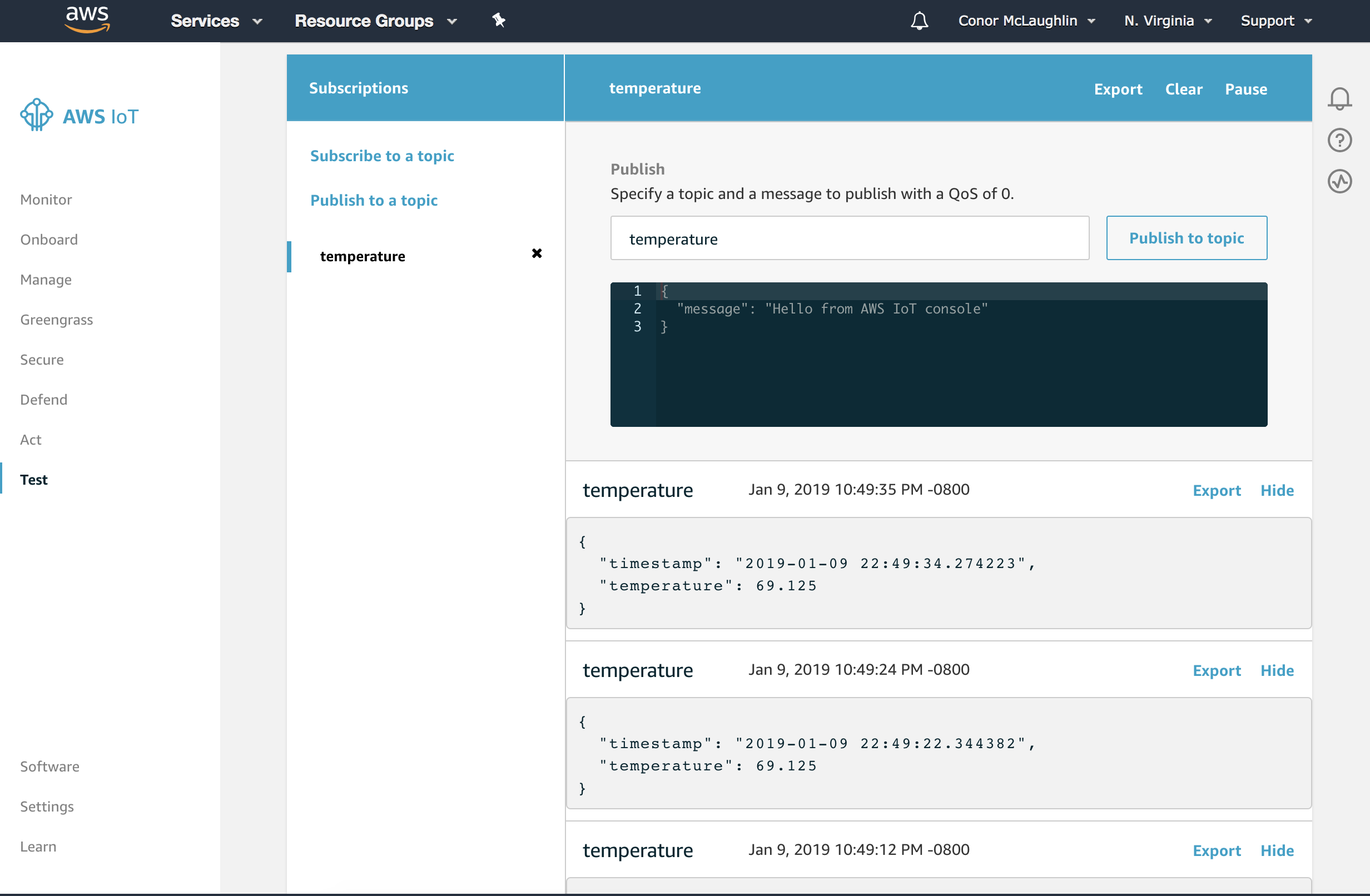
After testing that the code works, I recommend creating a job which runs on startup of your Raspberry Pi, and allows this Python script to always be running!

Connecting and Querying Athena within RStudio

Create AWS IoT Rules

Once you can see messages rolling into the proper topic in your AWS IoT hub, it’s time to start moving data around. The first thing you’ll want to do is create a rule which sends all messages to a Kinesis Firehose.

AWS IoT Rules

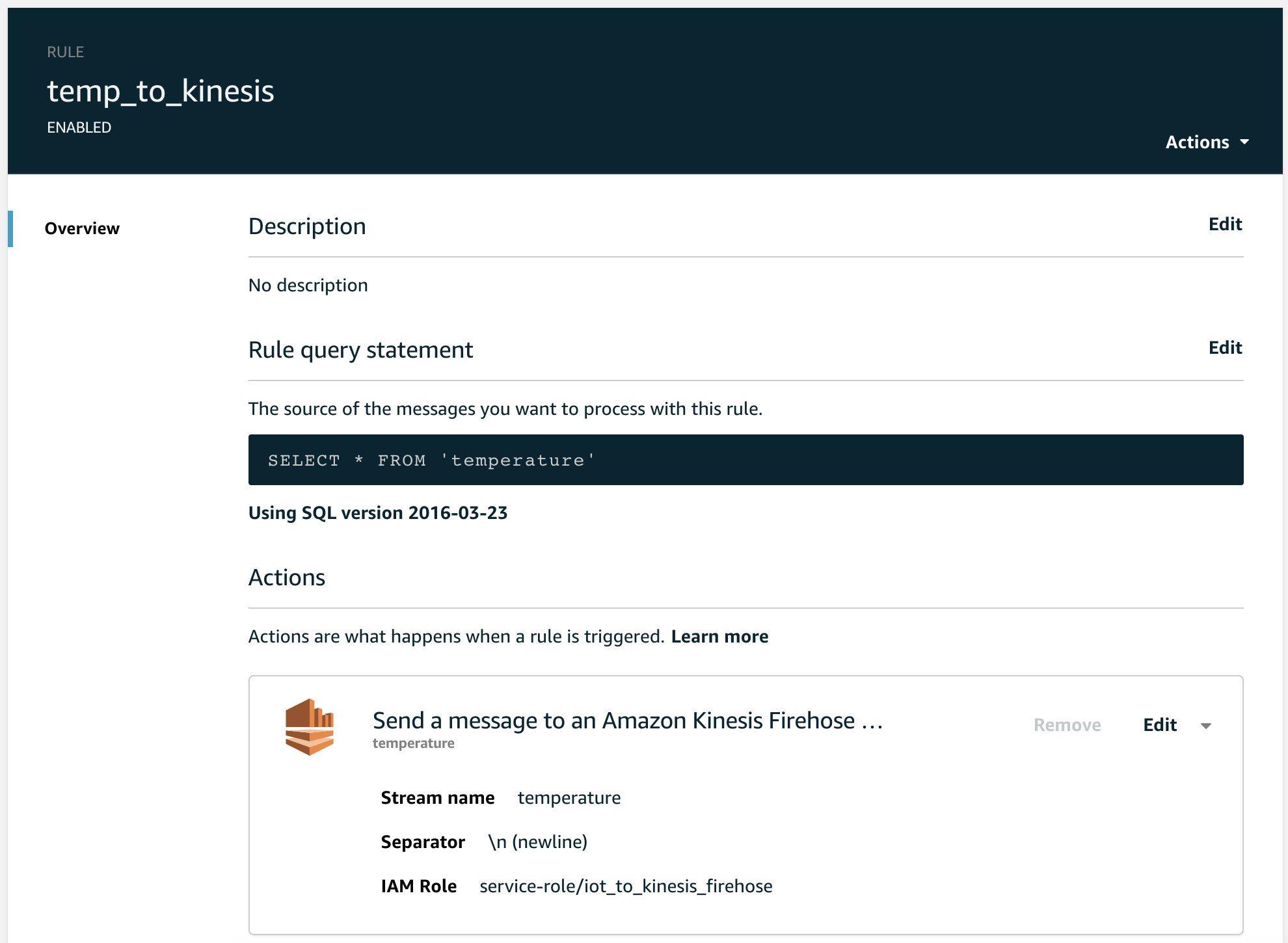
Create Kinesis Firehose Pipeline

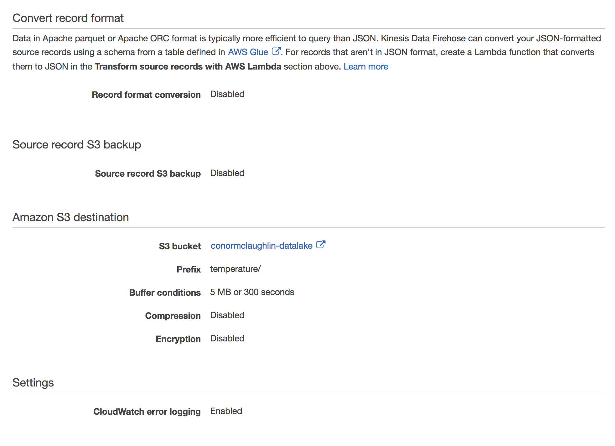
This should be a fairly automated process given the cues from the IoT setup, but bottom line is that here you’ll want to set up the writing of messages to S3. This is typically done in batches, and can be delivered to a bucket of your choosing.

Kinesis Firehose Setup

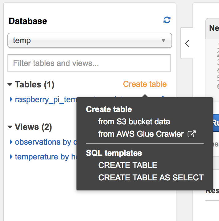
Connect Athena to your S3 Bucket

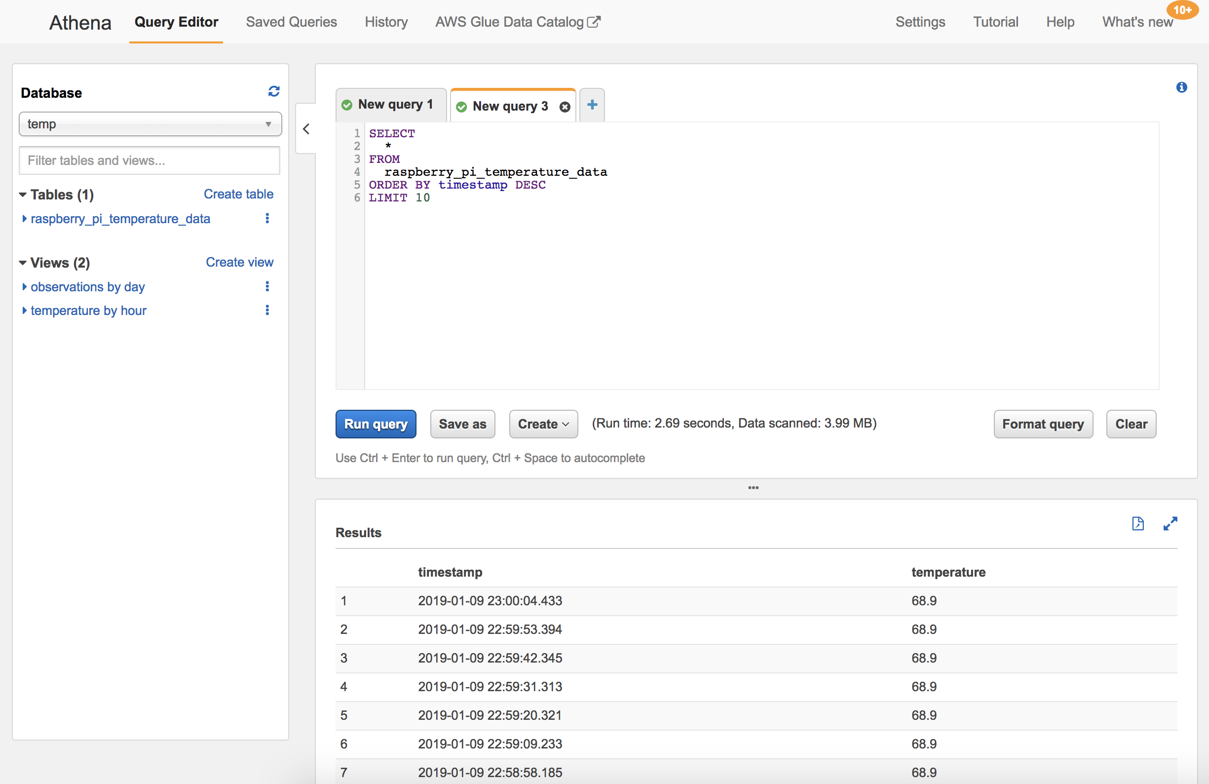
Once your data is being successfully output to the S3 bucket of your choosing, you can start using AWS Athena to query it. You’ll need to create a database, and then use the wizard to define a table based on your S3 bucket data.

Athena Create Table

Athena Query Interface

Run Athena Queries from RStudio

Once your data is queryable through Athena, you can connect to it using an RJDBC database connector and import the data into R and RStudio for further analysis. I chose to use the AMR.Athena package, which simplifies the connection and query process.

Here’s an example code snippet I utilized to query my data, which returns the average, minimum, and maximum temperatures per hour over the last week:

library(AWR.Athena)
library(rJava)
library(RJDBC)
require(DBI)

# Set up database connection to Athena
con <- dbConnect(AWR.Athena::Athena(), region='us-east-1', s3_staging_dir='s3://YOURBUCKETNAME', schema_name='default')
#dbListTables(con)

# Pull temp by hour for a week
week_temp <- dbGetQuery(con, 
                        "SELECT DATE_TRUNC('hour', timestamp) as hour, count(*) as observations, avg(temperature) as avg_temp, min(temperature) as min_temp, max(temperature) as max_temp
                        FROM temp.raspberry_pi_temperature_data
                        WHERE (date_trunc('day', timestamp) >= (date_trunc('day', current_timestamp - INTERVAL '8' HOUR) - INTERVAL '7' DAY))
                        GROUP BY 1
                        ORDER BY 1 DESC
                        ")

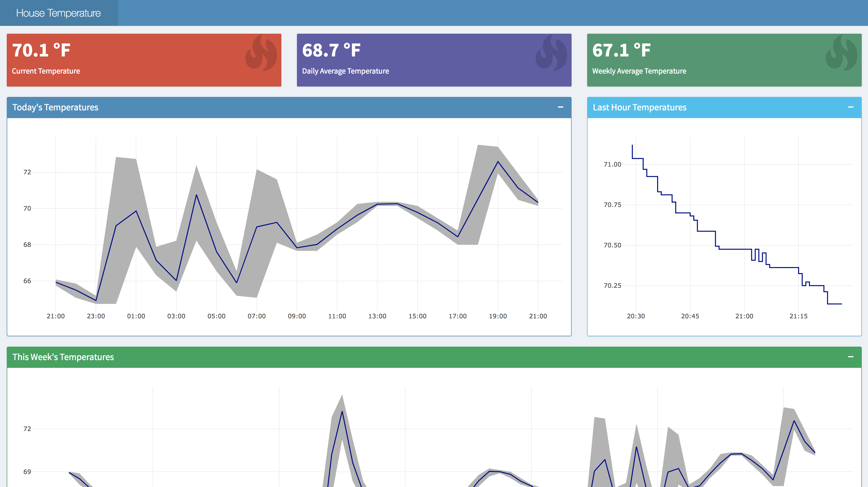
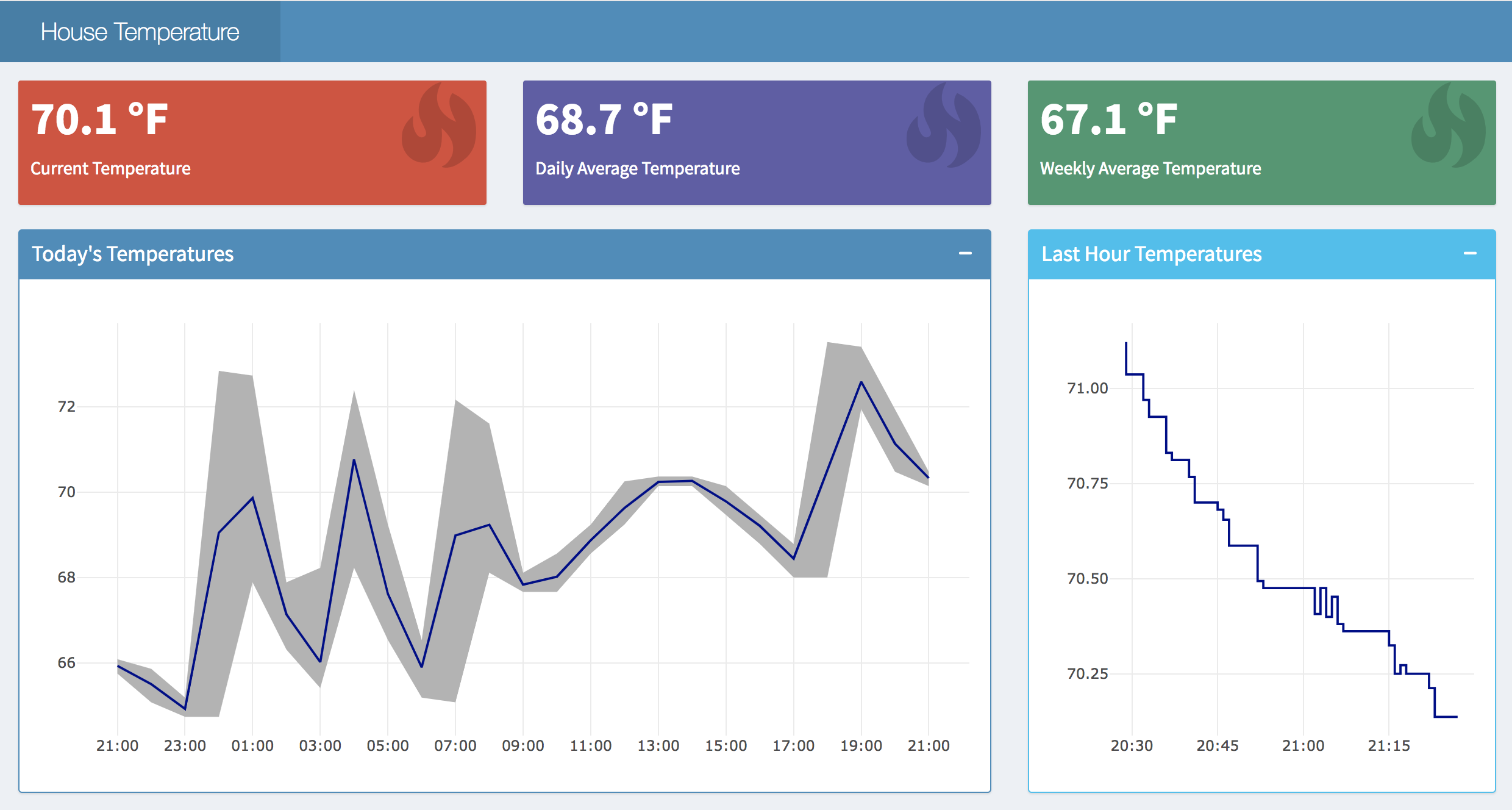
Visualizing Data

To visualize the different facets of the temperature data being returned, I built a Shiny Dashboard with a number of charts built in ggplot2 and Plotly. The application itself is broken into 3 parts:

ui.R: contains the simple scaffolding of the Shiny Dashboard
app.R: defines the server-side aspects of the Dashboard, such as the layout of boxes and plots, as well as their rendering
global.R: upon each run of the application, performs the relevant queries of the Athena database, and builds plots using the data it returns, which are later passed back to app.R to show in the app

ui.R

## ui.R ##
library(shinydashboard)

dashboardPage(
  dashboardHeader(),
  dashboardSidebar(),
  dashboardBody()
)

app.R

source('global.R', local = TRUE)

## app.R ##
library(shiny)
library(shinydashboard)
library(plotly)

ui <- dashboardPage(
  dashboardHeader(title = "House Temperature"),
  dashboardSidebar(disable = TRUE),
  dashboardBody(
    fluidRow(
      valueBoxOutput("now"),
      valueBoxOutput("day"),
      valueBoxOutput("week")
    ),
    fluidRow(
      box(
        plotlyOutput("d", height = 400), 
        title = "Today's Temperatures", 
        status = "primary", 
        solidHeader = TRUE,
        collapsible = TRUE,
        width = 8
        ),
      box(
        plotlyOutput("h", height = 400), 
        title = "Last Hour Temperatures", 
        status = "info", 
        solidHeader = TRUE,
        collapsible = TRUE,
        width = 4
      )
    ),
    fluidRow(
      box(
        plotlyOutput("w", height = 400), 
        title = "This Week's Temperatures", 
        status = "success", 
        solidHeader = TRUE,
        collapsible = TRUE,
        width = 12
      )
    )
  )
)

server <- function(input, output) { 
  output$now <- renderValueBox({
    valueBox(
      paste(round(last_temp$temperature, 1), "°F"), "Current Temperature", icon = icon("fire", lib = "glyphicon"),
      color = "red"
    )
  })
  
  output$day <- renderValueBox({
    valueBox(
      paste(round(mean(day_temp$avg_temp), 1), "°F"), "Daily Average Temperature", icon = icon("fire", lib = "glyphicon"),
      color = "purple"
    )
  })
  
  output$week <- renderValueBox({
    valueBox(
      paste(round(mean(week_temp$avg_temp), 1), "°F"), "Weekly Average Temperature", icon = icon("fire", lib = "glyphicon"),
      color = "olive"
    )
  })
  
  output$d <- renderPlotly({
    d
  })
  
  output$w <- renderPlotly({
    w
  }) 
  
  output$h <- renderPlotly({
    h
  }) 

}

shinyApp(ui, server)

global.R

library(tidyverse)
library(lubridate)
library(rJava)
library(RJDBC)
library(scales)
library(plotly)
library(AWR.Athena)
require(DBI)

# Set up database connection to Athena
con <- dbConnect(AWR.Athena::Athena(), region='us-east-1', s3_staging_dir='s3://YOURBUCKETNAME', schema_name='default')
#dbListTables(con)

# Note: all timestamps need to be adjusted given how our data is stored + UTC time on the database level
# Pull temp by hour for a week
week_temp <- dbGetQuery(con, 
                        "SELECT DATE_TRUNC('hour', timestamp) as hour, count(*) as observations, avg(temperature) as avg_temp, min(temperature) as min_temp, max(temperature) as max_temp
                        FROM temp.raspberry_pi_temperature_data
                        WHERE (date_trunc('day', timestamp) >= (date_trunc('day', current_timestamp - INTERVAL '8' HOUR) - INTERVAL '7' DAY))
                        GROUP BY 1
                        ORDER BY 1 DESC
                        ")
week_temp$hour <- ymd_hms(week_temp$hour)

# Pull temp by hour for 24 hour
day_temp <- dbGetQuery(con, 
                       "SELECT DATE_TRUNC('hour', timestamp) as hour, count(*) as observations, avg(temperature) as avg_temp, min(temperature) as min_temp, max(temperature) as max_temp
                       FROM temp.raspberry_pi_temperature_data
                       WHERE timestamp >= current_timestamp AT TIME ZONE 'America/Los_Angeles' - INTERVAL '32' HOUR
                       GROUP BY 1
                       ORDER BY 1 DESC
                       ")
day_temp$hour <- ymd_hms(day_temp$hour)

# Get the last recorded temp
last_temp <- dbGetQuery(con, 
                        "SELECT timestamp, temperature 
                        FROM temp.raspberry_pi_temperature_data
                        ORDER BY timestamp DESC
                        LIMIT 1
                        ")

# Pull temp by minute for last hour
hour_temp <- dbGetQuery(con, 
                        "SELECT DATE_TRUNC('minute', timestamp) as minute, count(*) as observations, avg(temperature) as avg_temp, min(temperature) as min_temp, max(temperature) as max_temp
                        FROM temp.raspberry_pi_temperature_data
                        WHERE timestamp >= current_timestamp - INTERVAL '9' HOUR
                        GROUP BY 1
                        ORDER BY 1 DESC
                        ")
hour_temp$minute <- ymd_hms(hour_temp$minute)

# Plot daily temp
d <- ggplot(day_temp, aes(x = hour, y = round(avg_temp,1))) + 
  geom_ribbon(aes(ymin = round(min_temp,1), ymax = round(max_temp, 1)), fill = "grey70") +
  geom_line(color = "darkblue") +
  labs(x = NULL, y = NULL) + 
  theme_minimal() +
  scale_x_datetime(labels = date_format("%H:00"), date_breaks = "2 hours", minor_breaks = "1 hours")
d <- ggplotly(d)

# Plot weekly temp
w <- ggplot(week_temp, aes(x = hour, y = avg_temp)) + 
  geom_ribbon(aes(ymin = min_temp, ymax = max_temp, fill = "grey70")) +
  geom_line(color = "darkblue") +
  labs(x = NULL, y = NULL) + 
  theme_minimal() +
  scale_x_datetime(labels = date_format("%b %d: %H:00"), date_breaks = "12 hours", minor_breaks = "6 hours")
w <- ggplotly(w)

# Plot hourly temp
h <- ggplot(hour_temp, aes(x = minute, y = avg_temp)) + 
  geom_step(color = "darkblue") +
  labs(x = NULL, y = NULL) + 
  theme_minimal() +
  scale_x_datetime(labels = date_format("%H:%M"))
h <- ggplotly(h)

Plots

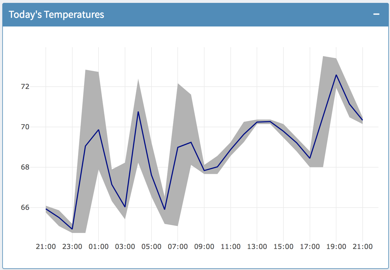
Today’s Temperature Plot

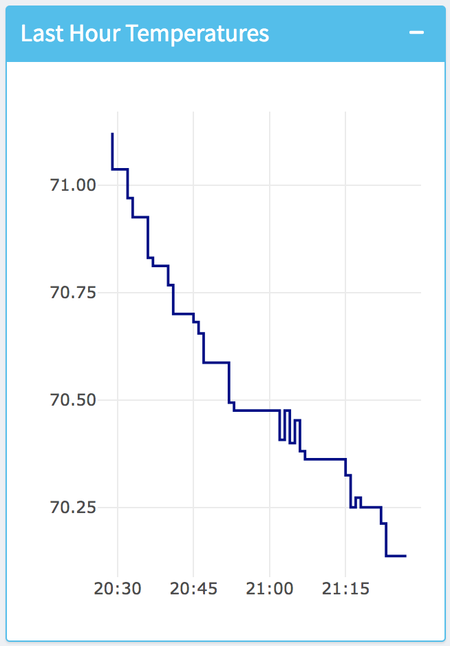
Last Hour’s Temperature Plot

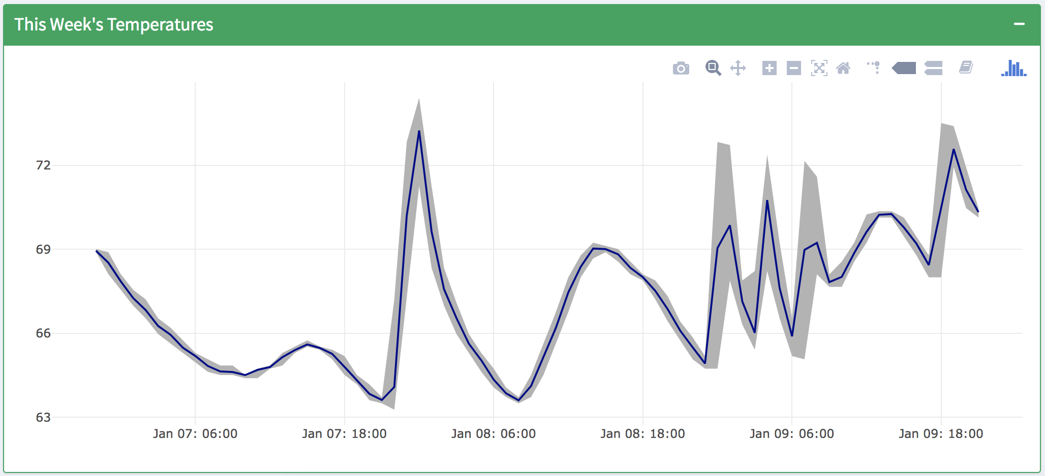
This Week’s Temperature Plot

Final Integrated Dashboard

The finished product looks good! I’m excited to be able to track trends in my house, and actually have a sense of when to crack a window or turn on the heat - I think there’s some fun work to be done on temperature forecasting, but that can wait for now.

Final Temperature Dashboard