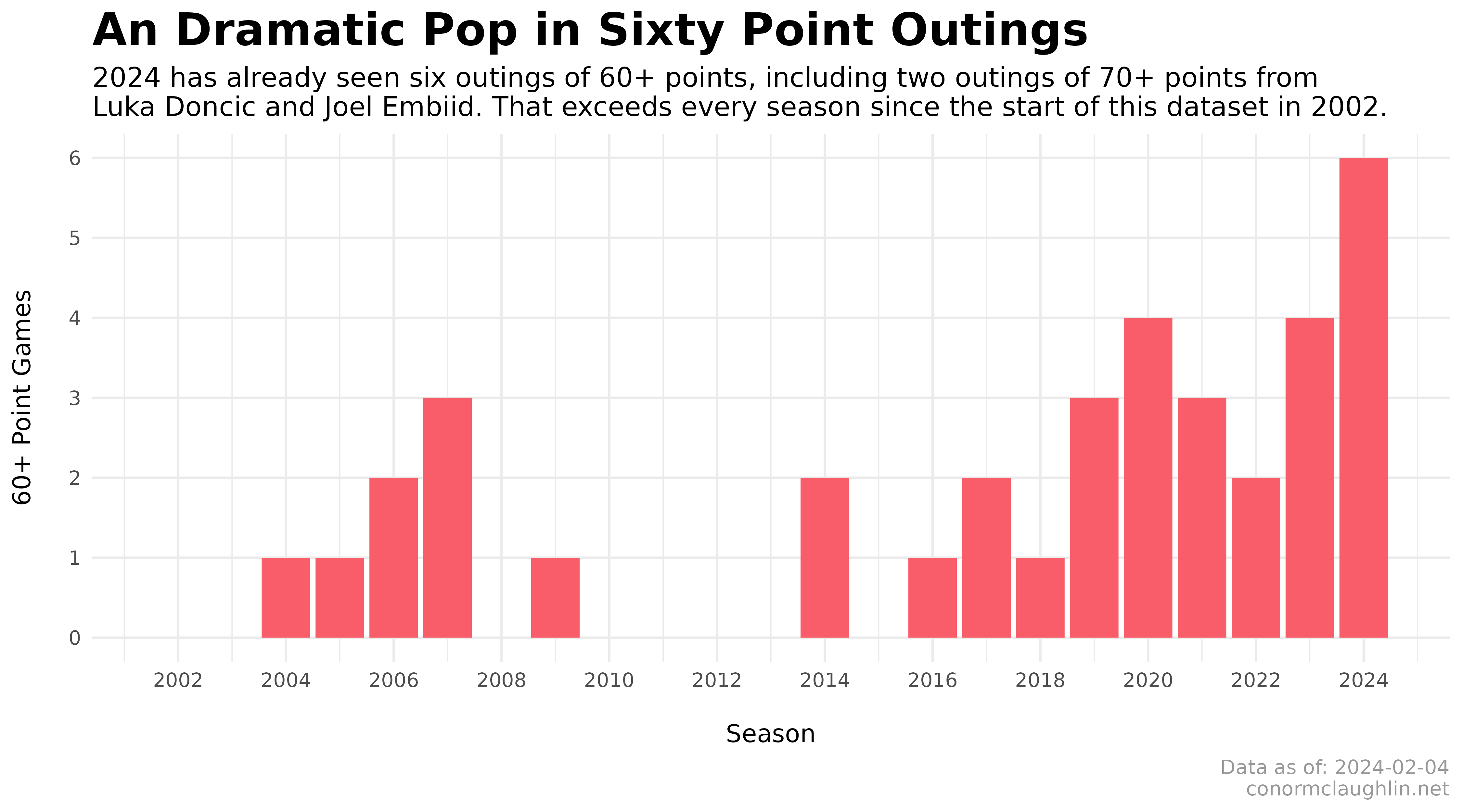
The past month of NBA basketball has been marked by a staggering amount of individual offensive brilliance, with Luka Doncic and Joel Embiid both going for 70 points, and Karl-Anthony Towns, Devin Booker, and Steph Curry all hitting the 60 point mark.
Prompted by this unique explosion of point scoring, I wanted to take a quick look at the history of high-scoring individual games, show how the recent events are really just the exclamation point on top of a long-term trend, and demonstrate how changes in the league’s offensive landscape have created a landscape more conducive to these outbursts.
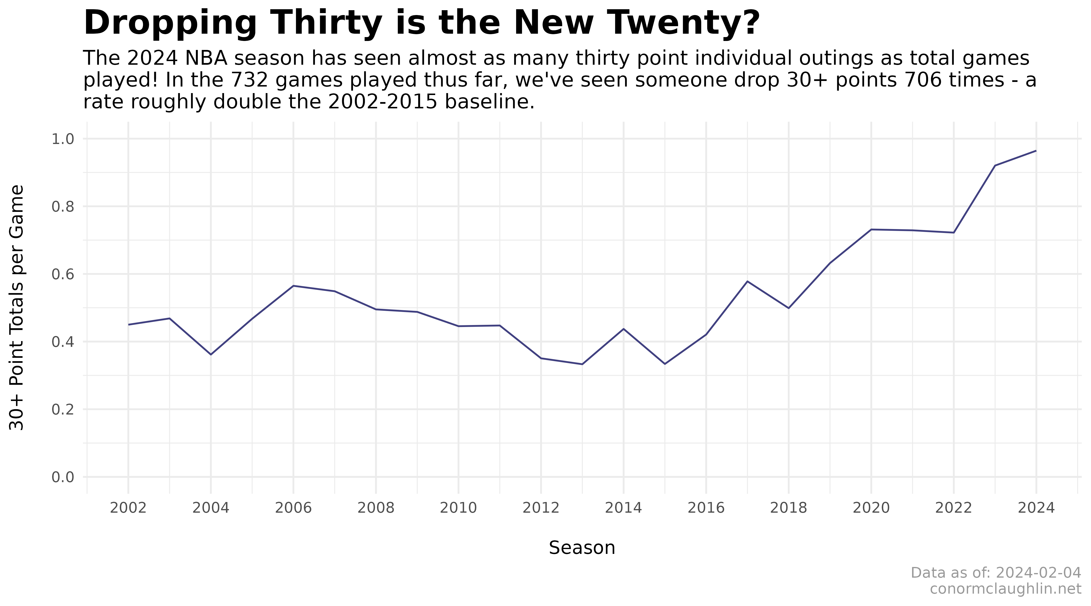
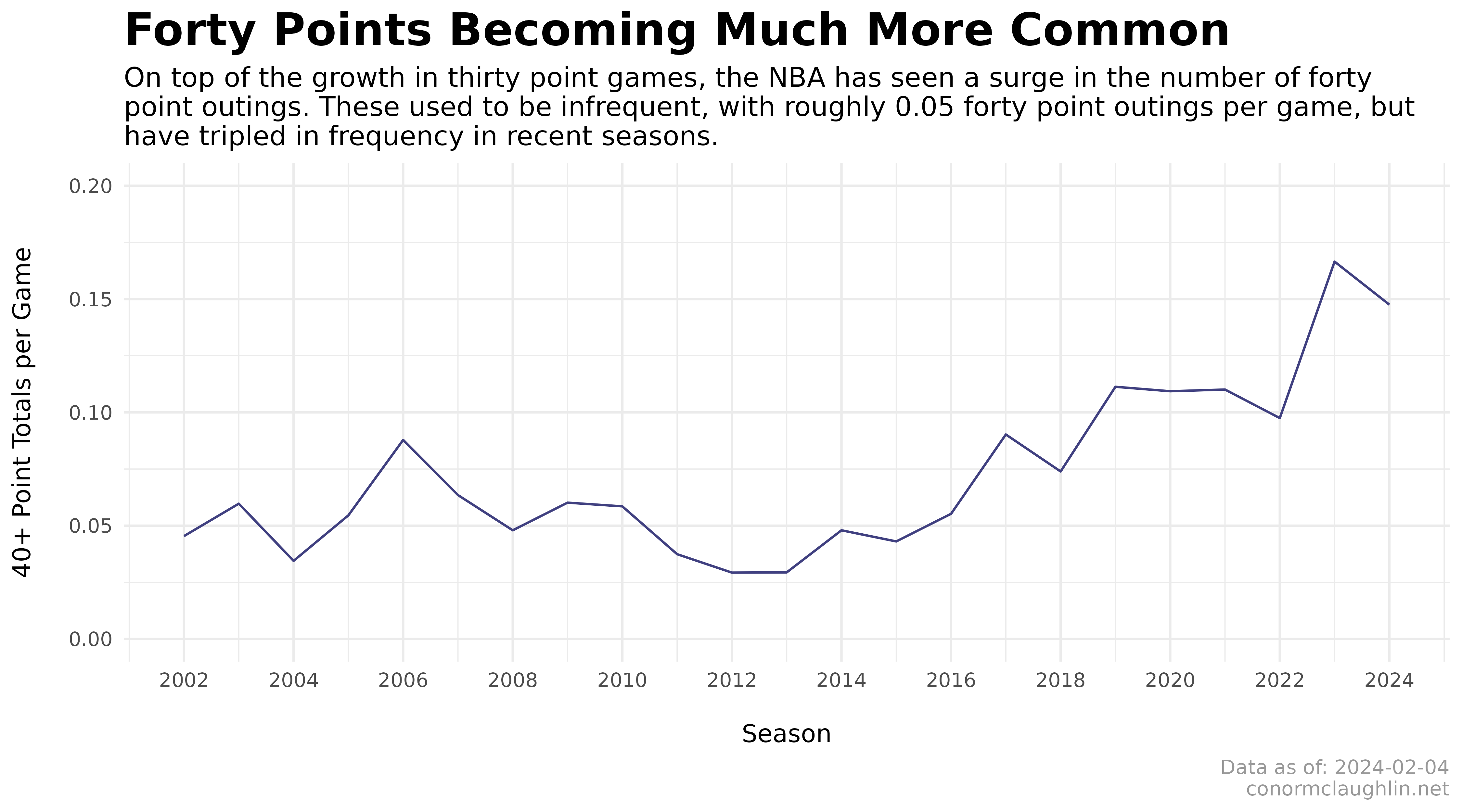
Frequency of High-Scoring Individual Games (30 and 40 Points)
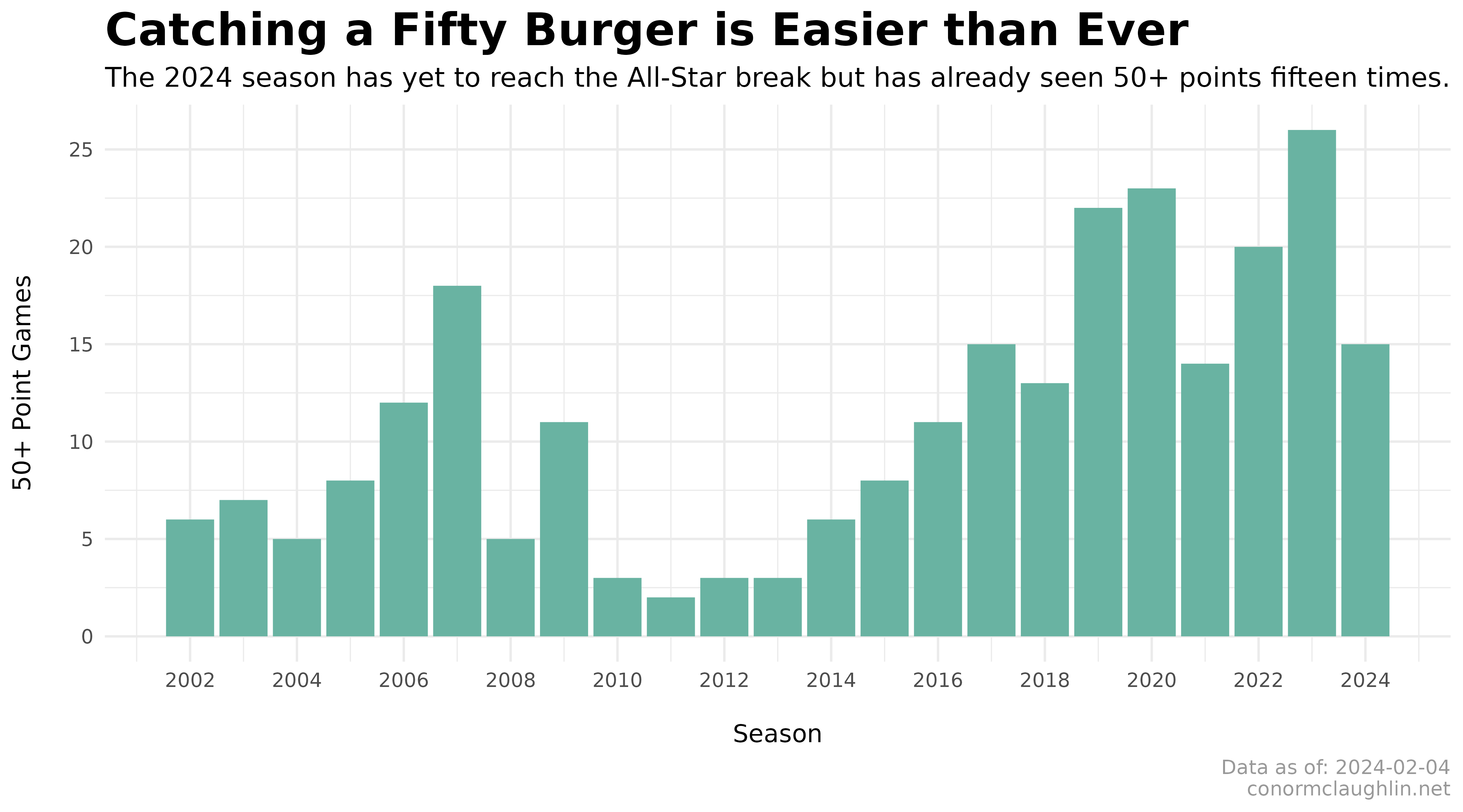
Volume of Extremely-High-Scoring Individual Games (50 and 60 Points)
What’s Driving The Increase in These Games?
There is a lot of conjecture about what’s driving the increase in high-scoring individual performances - a lack of defense, the refs, or the talent level of the young stars currently in the league.
While I’m sympathetic to each of those ideas, I generally think that these outbursts are a product of a league that has undergone a twenty year offensive evolution in which teams seek to play fast, maximize the number of high expected value (EV) shots (ie. 3s and layups), and minimize the number of low EV shots like midrange jumpers -> patterns which, in turn, raise the ceiling for any given individual player’s offensive output.
To test that hypothesis, I took a look into these league-wide offensive trends and found that they seem to support that judgement… Take a peek below!
Code Reference
I’d like to give a huge shoutout to the hoopR package for R which made it trivially easy to pull down 22 years of player box scores, allowing us to easily sort through the trends.
Sourcing NBA Player Box Scores
library(hoopR)
library(tidyverse)

nba_player_box <- load_nba_player_box(2002:most_recent_nba_season())
Look at 30/40/50 Point Frequency
df <- nba_player_box %>%
  filter(season_type == 2) %>%
  group_by(season) %>%
  summarize(
    points_30_per_game = sum(points >= 30, na.rm=TRUE) / n_distinct(game_id),
    points_40_per_game = sum(points >= 40, na.rm=TRUE) / n_distinct(game_id),
    points_50_per_game = sum(points >= 50, na.rm=TRUE) / n_distinct(game_id)
  )
Build 30 Point Frequency Chart
df %>%
  ggplot(aes(x = season, y = points_30_per_game)) +
    geom_line(color = "#404080") +
    expand_limits(y = c(0,1)) +
    scale_y_continuous(breaks = scales::pretty_breaks(6)) +
    scale_x_continuous(breaks = scales::pretty_breaks(9)) +
    theme_minimal() +
    theme(
      strip.background = element_rect(fill = "grey30"),
      strip.text = element_text(color = "grey97", face = "bold"),
      legend.background = element_rect(color = NA),
      plot.title = element_text(size = 20, face = "bold"),
      plot.subtitle = element_text(size = 12),
      plot.caption = element_text(colour = "grey60")
    ) +
    labs(
      x = "\nSeason",
      y = "30+ Point Totals per Game\n",
      title = "Dropping Thirty is the New Twenty?",
      subtitle = "The 2024 NBA season has seen almost as many thirty point individual outings as total games\nplayed! In the 732 games played thus far, we've seen someone drop 30+ points 706 times - a\nrate roughly double the 2002-2015 baseline.",
      caption = "Data as of: 2024-02-04\nconormclaughlin.net"
    )
Build League-Wide Statistics Graphic
library(reshape2)
nba_player_box %>%
filter(season_type == 2) %>%
group_by(season) %>%
summarize(
avg_team_score = mean(team_score),
fg_attempts = sum(field_goals_attempted, na.rm = TRUE) / n_distinct(game_id),
fg_pct = sum(field_goals_made, na.rm = TRUE) / sum(field_goals_attempted, na.rm = TRUE),
ft_attempts = sum(free_throws_attempted, na.rm = TRUE) / n_distinct(game_id),
ft_pct = sum(free_throws_made, na.rm = TRUE) / sum(free_throws_attempted, na.rm = TRUE),
two_pt_attempts = (sum(field_goals_attempted, na.rm = TRUE) - sum(three_point_field_goals_attempted, na.rm = TRUE)) / n_distinct(game_id),
two_pt_pct = (sum(field_goals_made, na.rm = TRUE) - sum(three_point_field_goals_made, na.rm = TRUE)) / (sum(field_goals_attempted, na.rm = TRUE) - sum(three_point_field_goals_attempted, na.rm = TRUE)),
three_pt_attempts = sum(three_point_field_goals_attempted, na.rm = TRUE) / n_distinct(game_id),
three_pt_pct = sum(three_point_field_goals_made, na.rm = TRUE) / sum(three_point_field_goals_attempted, na.rm = TRUE),
fouls = sum(fouls, na.rm = TRUE) / n_distinct(game_id),
turnovers = sum(turnovers, na.rm = TRUE) / n_distinct(game_id),
offensive_rebounds = sum(offensive_rebounds, na.rm = TRUE) / n_distinct(game_id),
) %>%
melt(id.vars = c("season")) %>%
ggplot(aes(x = season, y = value, group = variable, color = variable)) +
geom_line() +
scale_color_manual(
values = c(
"avg_team_score" = "#58508d",
"fg_attempts" = "#bc5090",
"two_pt_attempts" = "#bc5090",
"two_pt_pct" = "#bc5090",
"three_pt_attempts" = "#bc5090"
)
) +
facet_wrap(~ variable, scales = "free") +
theme_light() +
theme(
strip.background = element_rect(fill = "grey30"),
strip.text = element_text(color = "grey97", face = "bold"),
legend.background = element_rect(color = NA),
legend.position = "none",
plot.title = element_text(size = 20, face = "bold"),
plot.subtitle = element_text(size = 12),
plot.caption = element_text(colour = "grey60")
) +
labs(
x = "\nSeason",
y = "",
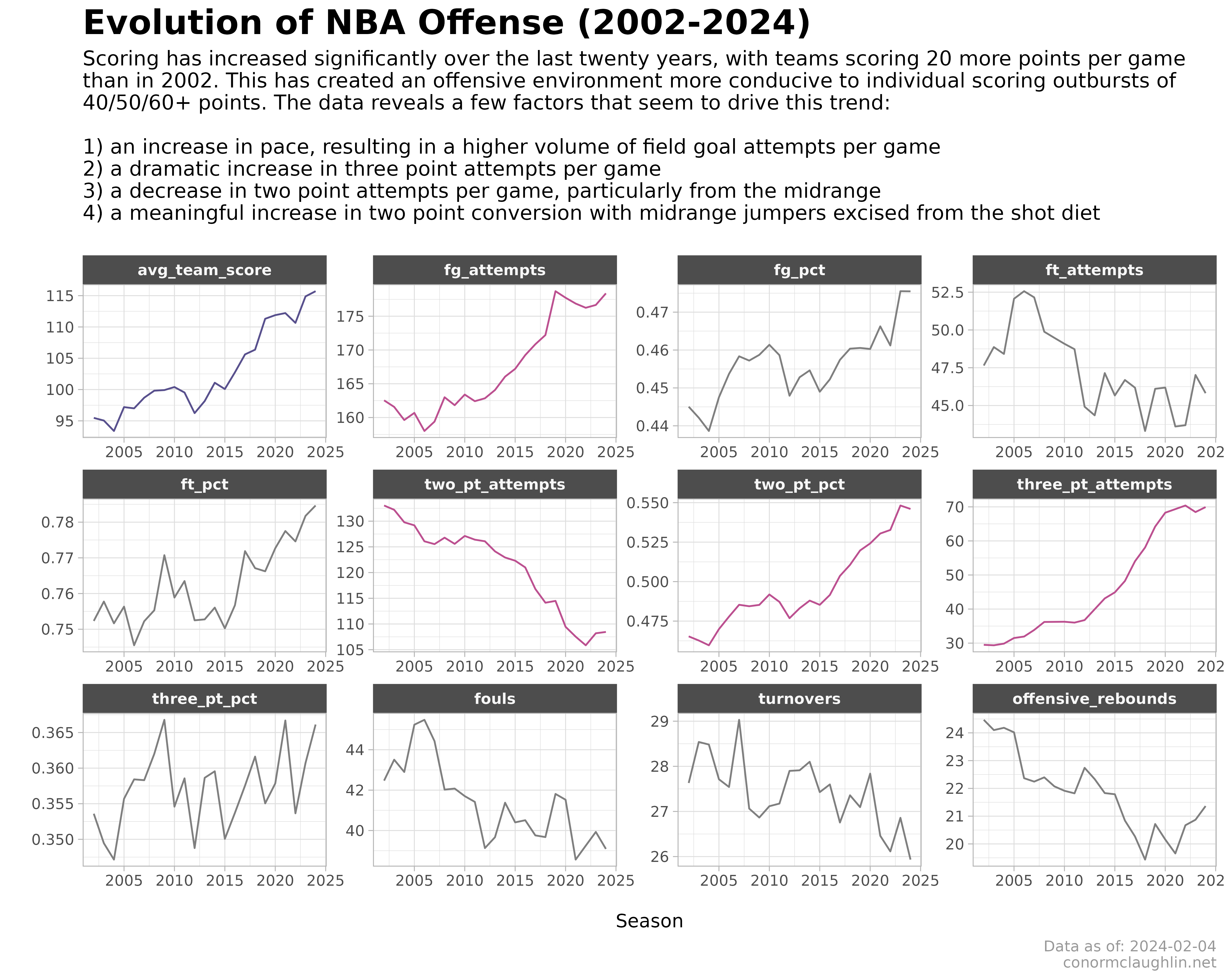
title = "Evolution of NBA Offense (2002-2024)",
subtitle = "Scoring has increased significantly over the last twenty years, with teams scoring 20 more points per game\nthan in 2002. This has created an offensive environment more conducive to individual scoring outbursts of\n40/50/60+ points. The data reveals a few factors that seem to drive this trend:\n\n1) an increase in pace, resulting in a higher volume of field goal attempts per game\n2) a dramatic increase in three point attempts per game\n3) a decrease in two point attempts per game, particularly from the midrange\n4) a meaningful increase in two point conversion with midrange jumpers excised from the shot diet\n",
caption = "Data as of: 2024-02-04\nconormclaughlin.net"
)