Santa Monica's Ocean Is Running Remarkably Warm

Anyone who has swum in the Pacific Ocean on the West Coast knows one thing - the water ain’t warm. Sure, it’s not quite as cold as Maine where my family goes in the summer… a trip that is very useful for me by making the California water seem “not that bad” upon my return! But the best adjectives in my experience have been “brisk” and “refreshing” - and you know what that means.

So, you can imagine my surprise when I popped in for a sunset swim a week or two ago and found the water to be downright pleasant! Compared to the usual experience of slowly edging my way into the water, then trying to build my courage for a dive into an oncoming wave, I was able to walk right in with zero hesitation. Something was obviously up, so after I got out of the ocean I checked the water temps and texted my family the semi-shocking number - it was 74 degrees!

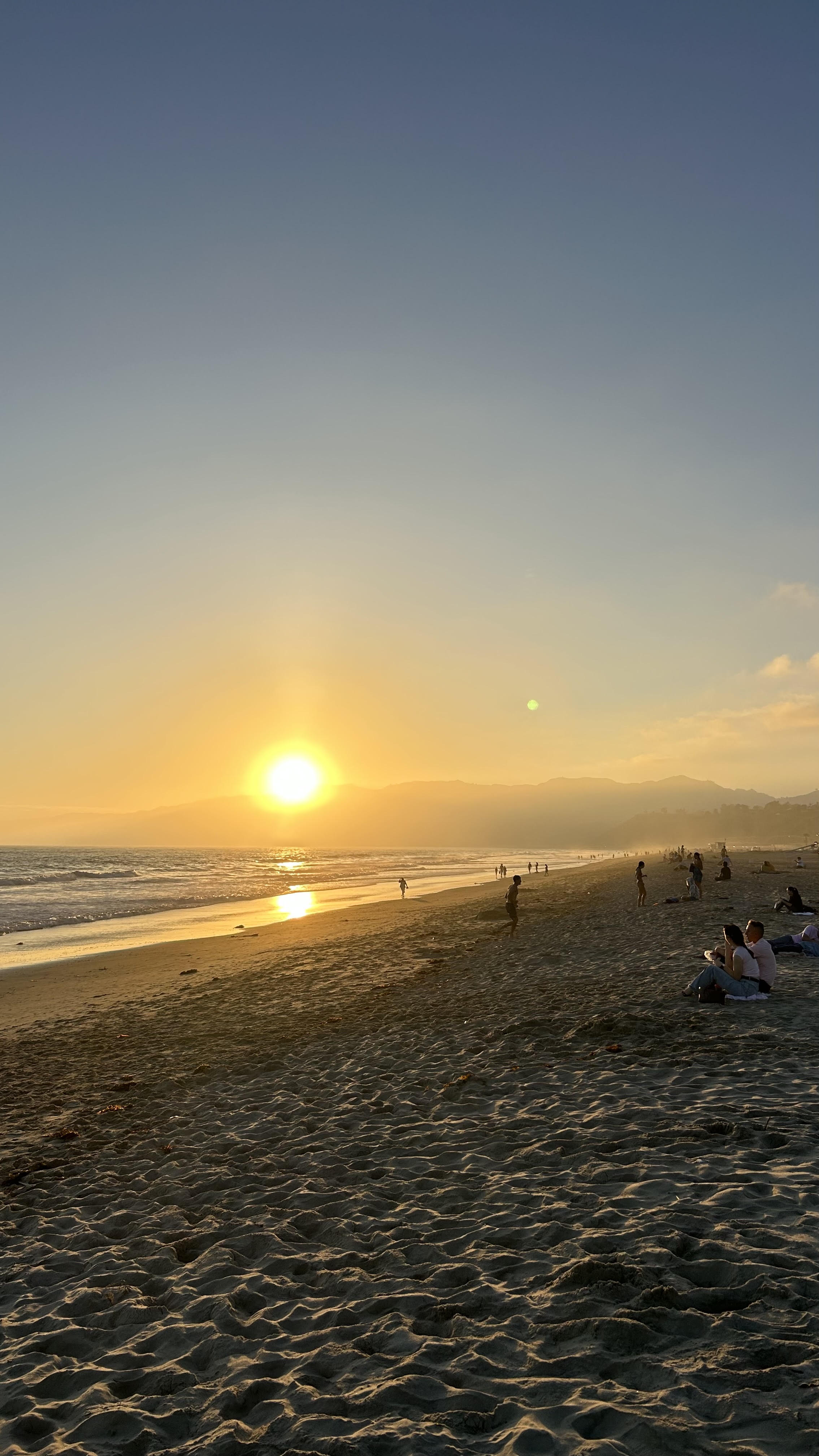
With that backdrop in mind (I’ve gone swimming several times in the past week to capitalize, don’t worry about me), I wanted to do a quick blog post highlighting this trend, which the data shows is truly anomalous.

Visualizing the Data

The water temperature at Santa Monica Pier has been running above its historical median for nearly all of 2026. The gap widened sharply in July, pushing the seven-day average beyond every comparable year in the station record.

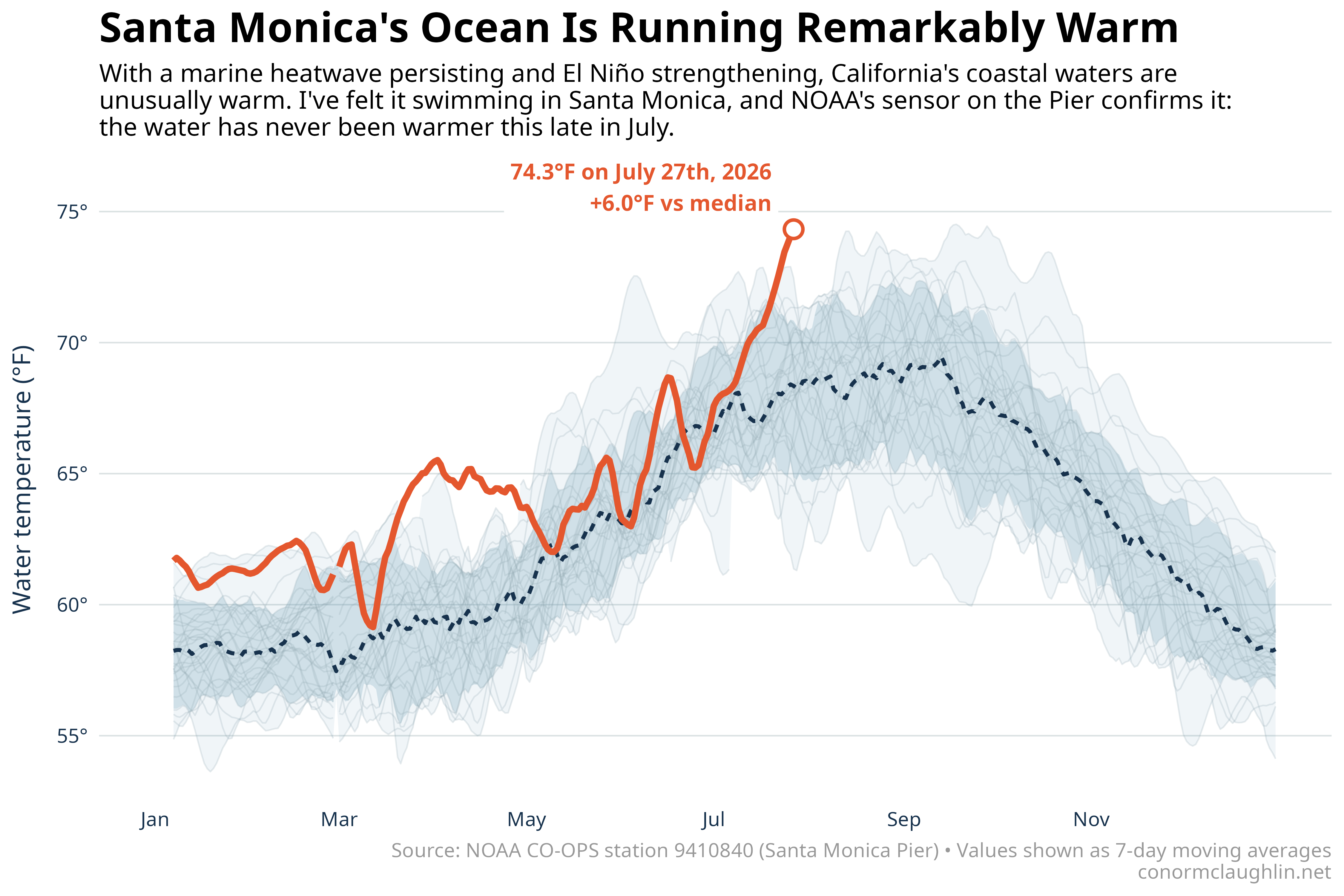
Through July 27, the rolling 7D average reached 74.3°F, roughly 6.0°F above the 1994–2025 median for the same point in the year. It was also 1.9°F warmer than the previous same-date high, recorded in 2003.

Averaging every available day from July 1 through July 27 produces the same conclusion: 2026 is the warmest July-to-date in the pier’s 33-year temperature record, narrowly ahead of 2018.

While the data is historic, there does seem to be fair reason for it - NOAA reports that a marine heatwave has persisted off central and Southern California, and the Climate Prediction Center says El Niño is active and strengthening. Those broader patterns set the stage for warmer water everywhere - I expect this trend in Santa Monica is emblematic of beach communities up and down the coast.

Code Reference

A Note on the Data

The source is NOAA CO-OPS station 9410840, located at Santa Monica Pier. Its water-temperature record begins in September 1993. The sensor sits 9.3 feet below mean lower low water, so these readings represent subsurface conditions at the pier rather than beach-wide surface temperature.

I converted NOAA’s hourly observations into local daily means, requiring at least 12 quality-screened readings for a day to count. The plotted values are trailing seven-day means, which smooth out day/night and tidal variation while preserving the larger warm spells.

Fetch Hourly Water Temperatures from NOAA

The NOAA CO-OPS Data API limits hourly requests to one year, so I fetched the record one calendar year at a time and combined the responses.

library(tidyverse)
library(jsonlite)
library(lubridate)

station_id <- "9410840"

get_water_temperature <- function(year) {
  end_date <- min(as.Date(sprintf("%d-12-31", year)), Sys.Date())

  url <- paste0(
    "https://api.tidesandcurrents.noaa.gov/api/prod/datagetter",
    "?product=water_temperature&application=conormclaughlin_blog",
    "&begin_date=", sprintf("%d0101", year), 
    "&end_date=", format(end_date, "%Y%m%d"),
    "&station=", station_id, "&time_zone=gmt",
    "&units=english&interval=h&format=json"
  )

  response <- fromJSON(url)

  response$data %>%
    transmute(
      timestamp_utc = as.POSIXct(t, format = "%Y-%m-%d %H:%M", tz = "UTC"),
      temperature_f = as.numeric(v),
      quality_flag = f
    )
}

hourly <- map_dfr(1993:year(Sys.Date()), get_water_temperature) %>%
  arrange(timestamp_utc) %>%
  distinct(timestamp_utc, .keep_all = TRUE)

Build Daily and Seven-Day Means

NOAA timestamps are returned in UTC. I converted them to Los Angeles time before assigning each observation to a calendar day.

trailing_mean <- function(x, n = 7L) {
  as.numeric(stats::filter(x, rep(1 / n, n), sides = 1))
}

season_day <- function(x) {
  as.integer(
    as.Date(paste0("2000-", format(as.Date(x), "%m-%d"))) -
      as.Date("2000-01-01")
  ) + 1L
}

daily <- hourly %>%
  mutate(
    timestamp_local = with_tz(timestamp_utc, "America/Los_Angeles"),
    local_date = as.Date(timestamp_local),
    flag_good = substr(quality_flag, 1, 1) == "0"
  ) %>%
  filter(flag_good, is.finite(temperature_f)) %>%
  group_by(local_date) %>%
  summarise(
    n_hours = n(),
    temperature_f = mean(temperature_f),
    .groups = "drop"
  ) %>%
  complete(local_date = seq(min(local_date), max(local_date), by = "day")) %>%
  mutate(
    temperature_f = if_else(n_hours >= 12, temperature_f, NA_real_),
    year = year(local_date),
    season_day = season_day(local_date),
    month_day = format(local_date, "%m-%d")
  ) %>%
  group_by(year) %>%
  arrange(local_date, .by_group = TRUE) %>%
  mutate(temperature_7day_f = trailing_mean(temperature_f, 7L)) %>%
  ungroup()

Calculate the Historical Range

I used 1994–2025 as the historical reference period because 1993 only contains observations beginning in September. Aligning on month and day also keeps leap years from shifting every date after February.

reference <- daily %>%
  filter(between(year, 1994, 2025), !is.na(temperature_7day_f))

climatology <- reference %>%
  group_by(season_day, month_day) %>%
  summarise(
    historical_median_f = median(temperature_7day_f),
    historical_p10_f = quantile(temperature_7day_f, 0.10),
    historical_p90_f = quantile(temperature_7day_f, 0.90),
    historical_min_f = min(temperature_7day_f),
    historical_max_f = max(temperature_7day_f),
    .groups = "drop"
  )

current_year <- daily %>%
  filter(year == 2026, !is.na(temperature_7day_f))