This week featured one of the most “NFC Least” matchups we’ve had in a while - an ugly 27-10 win by the Washington Commanders over the Philadelphia Eagles.
It brings me tremendous joy, of course, to see bad things happen to the Eagles (whose coach has no business being in the National Football League) - and I’ve been heartened by the fight the Commanders have shown in the second halves of recent games.
But what prompts me to write this post is a situation I noticed both squads kept ending up in: very long third downs. Throughout the game, it felt like every third down snap took place with eight or nine yards to the sticks… so after the game, I did a little exploration to see if the data supported my thinking.
Spoiler alert? It totally does - let’s take a peek below.
Third Down Trends
The simplest view of the data is often the most intuitive, what I built first was a scatterplot of Yards to Go vs Conversion Rate by team through the first eight weeks of the NFL season.
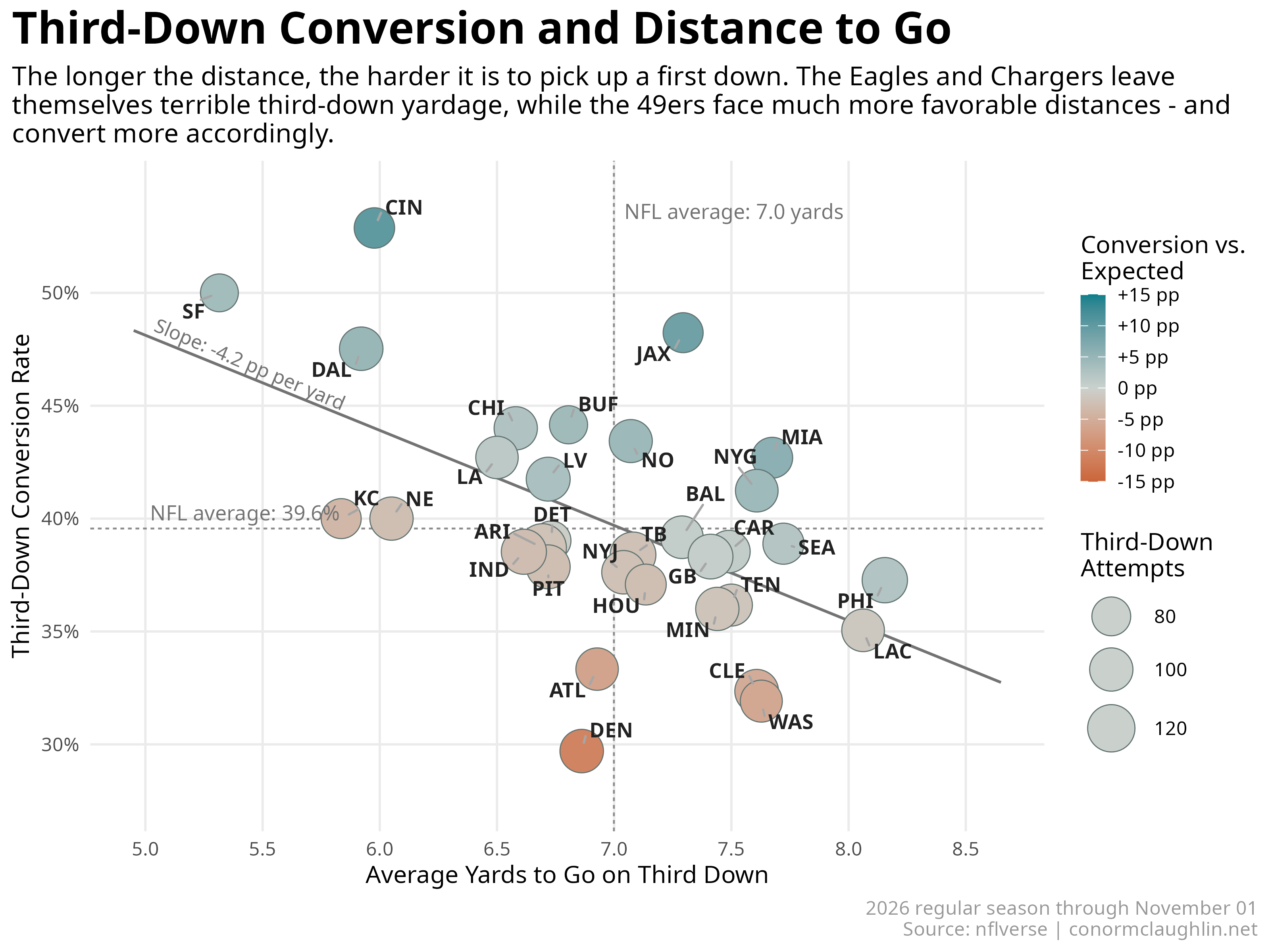
A few trends immediately jump out:
- There is a clear negative relationship between
Yards to GoandConversion Rate- each yard to go reducesConversion Rateby 4.2 ppts (R2 of 0.3, not bad)- I’ve added a hue dimension to the chart to illustrate how each team’s actual
Conversion Ratecompares to the Expected Rate, which is proxied by the line of best fit
- I’ve added a hue dimension to the chart to illustrate how each team’s actual
- The Niners, maybe the best team in the league so far, have clearly put themselves in the best third down positions and consequently convert 50% of the time, second to only the Bengals
- We can confirm that the Eagles are leaving themselves in dreadful shape on third downs - their average
Yards to Goof 8.2 is the worst in the league - The Commanders see slightly shorter yardage at 7.6 but actually convert worse than the Eagles do, with the data showing them better than only the (terribly boring) Denver Broncos on third
- Finally, the Jaguars are very meaningfully over-performing on third downs with +9 ppt of Conversion vs Expected, despite facing slightly longer-than-average distances
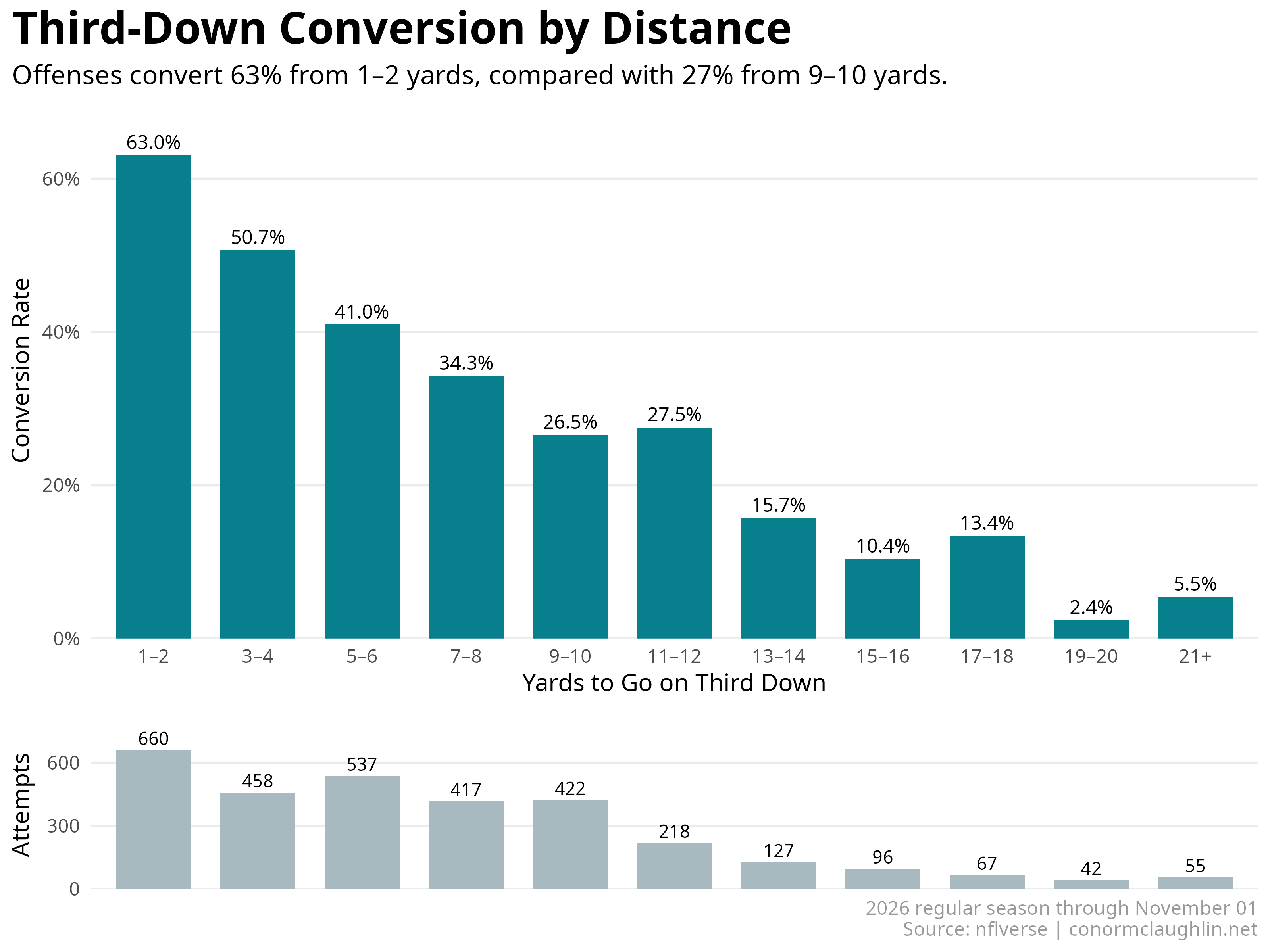
If we roll up all the team results and simply view conversion as a function of distance, we get a really clean dropoff curve that illustrates just how important it is to be in a third-and-short versus even a “third-and-manageable”:
Code Reference
This data was fetched from nflverse’s play-by-play data for the first eight weeks of the season.
Retrieve Plays
library(dplyr)

pbp <- nflreadr::load_pbp(2026, file_type = "csv")

third_downs <- pbp %>%
  filter(
    season == 2026,
    season_type == "REG",
    as.Date(game_date) <= as.Date("2026-11-01"),
    down == 3,
    third_down_converted == 1 | third_down_failed == 1
  ) %>%
  mutate(model_distance = log1p(pmin(ydstogo, 20)))
Compute Conversion against Expectation
third_downs$expected <- NA_real_

for (team in unique(third_downs$posteam)) {
  other_teams <- third_downs %>% filter(posteam != team)

  model <- glm(
    third_down_converted ~ splines::ns(model_distance, df = 3),
    data = other_teams,
    family = binomial()
  )

  team_rows <- which(third_downs$posteam == team)
  third_downs$expected[team_rows] <- predict(
    model, newdata = third_downs[team_rows, ], type = "response"
  )
}
Summarize Each Offense
teams <- third_downs %>%
  group_by(team = posteam) %>%
  summarise(
    attempts = n(),
    conversions = sum(third_down_converted),
    conversion_rate = mean(third_down_converted),
    mean_yards_to_go = mean(ydstogo),
    expected_rate = mean(expected),
    .groups = "drop"
  ) %>%
  mutate(above_expected_pp = 100 * (conversion_rate - expected_rate)) %>%
  arrange(desc(above_expected_pp))
Build the Scatterplot
library(ggplot2)
library(ggrepel)

linear_fit <- lm(conversion_rate ~ mean_yards_to_go, data = teams)
linear_slope <- coef(linear_fit)[2]

ggplot(teams, aes(mean_yards_to_go, conversion_rate)) +
  geom_smooth(
    method = "lm", formula = y ~ x, se = FALSE, fullrange = TRUE,
    colour = "grey45", linewidth = 0.6, alpha = 0.65
  ) +
  geom_point(
    aes(size = attempts, fill = above_expected_pp),
    shape = 21, colour = "grey45"
  ) +
  geom_text_repel(aes(label = team), seed = 2026) +
  annotate(
    "text", x = 5.02,
    y = unname(coef(linear_fit)[1] + 5.02 * linear_slope),
    label = sprintf("Slope: %.1f pp per yard", 100 * linear_slope),
    angle = -23, hjust = 0, vjust = -0.5, colour = "grey45", size = 3.1
  ) +
  scale_fill_gradient2(
    low = "#CB653A", mid = "#CAD1CD", high = "#087F8C",
    midpoint = 0, limits = c(-15, 15),
    breaks = seq(-15, 15, 5),
    labels = function(x) paste0(ifelse(x == 0, "0", sprintf("%+d", x)), " pp"),
    name = "Conversion vs.\nExpected"
  ) +
  scale_size_area(max_size = 10, name = "Third-Down Attempts") +
  scale_y_continuous(labels = scales::label_percent()) +
  theme_minimal() +
  theme(
    plot.title = element_text(size = 20, face = "bold"),
    plot.subtitle = element_text(size = 12),
    plot.caption = element_text(colour = "grey60"),
    plot.title.position = "plot",
    legend.position = "right"
  ) +
  labs(
    title = "Third-Down Conversion and Distance to Go",
    x = "Average Yards to Go on Third Down",
    y = "Third-Down Conversion Rate",
    caption = "2026 regular season through November 1\nSource: nflverse | conormclaughlin.net"
  )
Build the Distance-Band Chart
I grouped attempts into two-yard bands through 20 yards, with the remaining attempts pooled into 21+. The smaller panel below shows how many attempts fall into each band.
library(scales)
library(grid)

bands <- third_downs %>%
  mutate(band_start = pmin(2 * floor((ydstogo - 1) / 2) + 1, 21)) %>%
  group_by(band_start) %>%
  summarise(
    attempts = n(),
    conversion_rate = mean(third_down_converted),
    .groups = "drop"
  ) %>%
  arrange(band_start) %>%
  mutate(
    distance_band = if_else(band_start == 21, "21+",
                           paste0(band_start, "–", band_start + 1)),
    distance_band = factor(distance_band, levels = distance_band)
  )
Both panels share the same distance bands, with the labels directly underneath the conversion bars.
band_theme <- theme_minimal() +
  theme(
    panel.grid.major.x = element_blank(),
    panel.grid.minor = element_blank(),
    plot.title = element_text(size = 20, face = "bold"),
    plot.subtitle = element_text(size = 12),
    plot.caption = element_text(colour = "grey60"),
    plot.title.position = "plot",
    plot.caption.position = "plot"
  )

rates <- ggplot(bands, aes(distance_band, conversion_rate)) +
  geom_col(fill = "#087F8C", width = 0.72) +
  geom_text(aes(label = percent(conversion_rate, accuracy = 0.1)),
            vjust = -0.45, size = 3.1) +
  scale_y_continuous(
    labels = label_percent(accuracy = 1), breaks = seq(0, 0.6, 0.2),
    limits = c(0, 0.7), expand = expansion(mult = c(0, 0))
  ) +
  labs(
    title = "Third-Down Conversion by Distance",
    subtitle = "Offenses convert 63% from 1–2 yards, compared with 27% from 9–10 yards.",
    x = "Yards to Go on Third Down", y = "Conversion Rate"
  ) +
  band_theme + theme(plot.margin = margin(5.5, 5.5, 8, 5.5))

volume <- ggplot(bands, aes(distance_band, attempts)) +
  geom_col(fill = "#A8B9C0", width = 0.72) +
  geom_text(aes(label = comma(attempts)), vjust = -0.4, size = 2.9) +
  scale_y_continuous(
    breaks = c(0, 300, 600), limits = c(0, 800),
    expand = expansion(mult = c(0, 0))
  ) +
  labs(
    x = NULL, y = "Attempts",
    caption = "2026 regular season through November 1\nSource: nflverse | conormclaughlin.net"
  ) +
  band_theme +
  theme(
    axis.text.x = element_blank(), axis.ticks.x = element_blank(),
    plot.margin = margin(3, 5.5, 5.5, 5.5)
  )
Matching the panel widths keeps the bars aligned. The conversion chart gets three-quarters of the height, leaving a compact strip for volume.
rates_grob <- ggplotGrob(rates)
volume_grob <- ggplotGrob(volume)
shared_widths <- unit.pmax(rates_grob$widths, volume_grob$widths)
rates_grob$widths <- shared_widths
volume_grob$widths <- shared_widths

panels <- grobTree(
  editGrob(rates_grob, name = "rate_panel",
           vp = viewport(x = 0.5, y = 0.625, width = 1, height = 0.75)),
  editGrob(volume_grob, name = "volume_panel",
           vp = viewport(x = 0.5, y = 0.125, width = 1, height = 0.25))
)

grid.newpage()
grid.draw(panels)